01-Downloading patches from Google Earth Engine
Google Earth Engine (GEE) is a geospatial processing service. GEE allows users to run algorithms on georeferenced imagery and vectors stored on Google's infrastructure. The GEE API provides a library of functions which may be applied to data for display and analysis.With Earth Engine, you can perform geospatial processing at scale, powered by Google Cloud Platform. The purpose of Earth Engine is to:
- Provide an interactive platform for geospatial algorithm development at scale
- Enable high-impact, data-driven science
- Make substantive progress on global challenges that involve large geospatial datasets
01. Libraries to be used:
| import ee
import geemap as emap
|
02. Authentication and Initialization
Prior to using the Earth Engine Python client library, you need to authenticate and use the resultant credentials to initialize the Python client. To initialize, you will need to provide a project that you own, or have permissions to use. This project will be used for running all Earth Engine operations:
| ee.Authenticate()
ee.Initialize(project='ee-geoyons')
|
See the authentication guide for troubleshooting and to learn more about authentication modes and Cloud projects.
Selecting a specific basemap as follow:
| Map = emap.Map()
Map.add_basemap("SATELLITE")
|
03. Downloading patches from GEE and Python
Patches for Deep Learning architectures are crucial for land cover disturbance mapping, including burned area mapping. A good option is to download from GEE using the Python API or JavaScript, whichever you are comfortable with. In this tutorial, the Python API will be used to stay within the Google Colab environment.
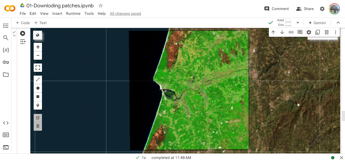
A specific tile with 50x50km (i.e., 25 million pixels) from Portugal during the 2017 year will be downloaded. Labeling data known as ground truth for the same tile will be downloaded as well.
Let's work on coding.
1
2
3
4
5
6
7
8
9
10
11
12
13
14
15
16
17
18
19
20
21
22
23
24
25
26
27
28
29
30
31
32
33
34
35
36
37
38
39
40
41
42
43
44
45
46
47
48
49
50
51
52
53
54
55
56
57
58
59
60
61
62
63
64
65
66
67
68
69
70
71
72
73
74
75
76
77 | # specific tile to be used
tile = ee.List([17])
# tiles for Portugal
port_tiles = ee.FeatureCollection("projects/ee-geoyons/assets/tiles_portugal_50km")
# labeling data - burned area during the 2017 year
label = ee.Image("projects/ee-geoyons/assets/raster_ardida_2017")
# selecting tile 17
features = port_tiles.filter(ee.Filter.inList('id', tile));
# define a collection
colS2 = 'COPERNICUS/S2_SR_HARMONIZED'
# NBR function
def addNBR (image):
nbr = image.normalizedDifference(['B8', 'B12']).rename("NBR");
return image.addBands(nbr);
# masking clouds
def maskSQA(image):
qa = image.select('QA60')
opaque_cloud = (1 << 10);
cirrus_cloud = (1 << 11);
mask = qa.bitwiseAnd(opaque_cloud).eq(0).And(qa.bitwiseAnd(cirrus_cloud).eq(0));
return image.updateMask(mask);
cloud_cover = 10;
bnames = ['B2', 'B3', 'B4', 'B5','B6','B7','B8','B8A','B11','B12']
### ********************************* AFTER THE EVENT ******************************
# dates AFTER the fire event
start_date_after = '2017-09-30';
end_date_after = '2017-12-30';
# base satellite image as input for burned area
img2017 = ee.ImageCollection(colS2)\
.filterBounds(features)\
.filterDate(start_date_after, end_date_after)\
.filter(ee.Filter.lt('CLOUDY_PIXEL_PERCENTAGE', cloud_cover))\
.map(maskSQA)\
.select(bnames)\
.reduce(ee.Reducer.median())
# NBR collection computed
nbrColl = ee.ImageCollection(colS2)\
.filterBounds(features)\
.filterDate(start_date_after, end_date_after)\
.filter(ee.Filter.lt('CLOUDY_PIXEL_PERCENTAGE', cloud_cover))\
.map(maskSQA)\
.select(bnames)\
.map(addNBR)\
.reduce(ee.Reducer.min());
# NBR after the event
nbr_after = nbrColl.select('NBR_min');
### ********************************* BEFORE THE EVENT ******************************
# dates BEFORE the fire event
start_date_before = '2020-09-30'; # '2017-04-01';
end_date_before = '2020-12-30'; # '2017-06-15'
# NBR collection computed
nbrColl2 = ee.ImageCollection(colS2)\
.filterBounds(features)\
.filterDate(start_date_before, end_date_before)\
.filter(ee.Filter.lt('CLOUDY_PIXEL_PERCENTAGE', 90))\
.map(maskSQA)\
.select(bnames)\
.map(addNBR)\
.reduce(ee.Reducer.mean());
# NBR before the event
nbr_before = nbrColl2.select('NBR_mean');
# dNBR
nbr_diff = nbr_after.subtract(nbr_before);
|
GEE has some visualization parameters for the Map.addLayer() function in order to enhance the image histogram values.

Courtesy: Qiusheng Wu
1
2
3
4
5
6
7
8
9
10
11
12
13
14
15
16
17
18
19
20
21 | # params for base image visualization
vizParams = {
"bands": ['B12_median', 'B8_median', 'B4_median'],
"min": 0,
"max": 3500,
"gamma": [0.95, 1.1, 1]
};
# params for NBR index
params_nbr = {
"min": -0.4,
"max": 0.6,
"palette": ['FFFFFF','CC9966','CC9900','996600', '33CC00', '009900','006600']};
Map.centerObject(features, 10)
Map.addLayer(features, {},'Portugal tiles', True);
Map.addLayer(img2017.clip(features), vizParams, 'S2 - Post-fire event 2017', True);
Map.addLayer(nbr_before.select('NBR_mean').clip(features), params_nbr, 'NBR before', True);
Map.addLayer(nbr_after.clip(features).select('NBR_min'), params_nbr, 'NBR after', True);
Map.addLayer(nbr_diff.clip(features), {'min': -0.9, 'max': 0.9}, 'NBR Difference (dNBR)', True);
Map
|
04. Downloading and exporting images
When you export an image, the data are ordered as channels, height, width (CHW). The export may be split into multiple TFRecord files with each file containing one or more patches of size patchSize, which is user specified in the export. The size of the files in bytes is user specified in the maxFileSize parameter.
The patchSize, maxFileSize, and kernelSize parameters are passed to the ee.Export (JavaScript) or ee.batch.Export (Python) call through a formatOptions dictionary, where keys are the names of additional parameters passed to Export. Possible formatOptions for an image exported to TFRecord format are on the official GEE documentation page.
We generated 512x512 pixel patches for both the 11 input variables (10 S2 bands + 1 dNBR) and the labeling data. Bands of Sentinel-2 used:
- B2 (Blue)
- B3 (Green)
- B4 (Red)
- B5 (Vegetation red edge 1)
- B6 (Vegetation red edge 2)
- B7 (Vegetation red edge 3)
- B8 (Near infrared)
- B8A (Vegetation red edge 4)
- B11 (SWIR1)
- B12 (SWIR2)
- dNBR (NBR difference)
- label (Labeling data)
1
2
3
4
5
6
7
8
9
10
11
12
13
14
15
16
17
18
19 | # formatOptions
formatOptions = {
'patchDimensions': [512, 512], #512*512
'maxFileSize': 104857600,
'compressed': True
}
# exporting patches to Google Drive
ee.batch.Export.image({
"image": img2017.clip(features).double(),
"description": 'PatchesExport',
"fileNamePrefix": 'Port_tile17',
"scale": 10, # spatial resolution
"folder": 'Portugal_patches_512-512_tile17',
"fileFormat": 'TFRecord',
"region": features,
"formatOptions": formatOptions,
"maxPixels": 1e+13,
})
|