04. Predicting large images
01. key variables
Let's first save some key variables that will be used for prediction and for reconstructing the whole image in a single patch.
 1
 2
 3
 4
 5
 6
 7
 8
 9
10
11
12 | # total patches
total_patches = mixer['totalPatches'] # 108
# patches per row
num_patches_rows = mixer['patchesPerRow'] # 12
# patches per col
num_patches_cols = total_patches // num_patches_rows # 9
# path size
patch_size = 512
# number of bands
nbands = 11
# Patches by rows and cols (integer)
print(f'number of patches in rows: {num_patches_rows}\nnumber of patches in cols: {num_patches_cols}')
|
02. N-dimensional Tensor
In this step, a 4-dimensional tensor of X will be reshaped to a 6-dimensional tensor, which means patches per col, patches per row, height of 1, path size, patch size, number of bands. Regarding the labelind data, it will be reshape to a 4-dimensional tensor, i.e., patches per col, patches per row, path size and patch size.
 1
 2
 3
 4
 5
 6
 7
 8
 9
10
11
12
13
14
15
16
17 | # reshape the image patches
patches = np.reshape(X, (num_patches_cols,
num_patches_rows,
patch_size,
patch_size,
nbands)) # 9, 12, 512,512,11
patches = np.expand_dims(patches, axis = 2)
print("Patches array shape is: ", patches.shape)
# reshape the labeling data patches
patches_labels = np.reshape(y, (num_patches_cols,
num_patches_rows,
patch_size,
patch_size)) # 9, 12, 512,512
print("Patches labeling shape is: ", patches_labels.shape)
|
03. Predicting the whole image: tile 17
In this step, patches as tensor will be used for prediction, then the predicted patches will be saved as a 4-dimensional tensor with patches per col, patches per row, path size and patch size.
 1
 2
 3
 4
 5
 6
 7
 8
 9
10
11
12
13
14
15
16
17 | # Apply the trained model on large image, patch by patch
predicted_patches = []
for i in range(num_patches_cols):
for j in range(num_patches_rows):
print("Now predicting on patch", i,j)
single_patch = patches[i,j,0,:,:,:]
single_patch_input = np.expand_dims(single_patch, axis = 0)
single_patch_prediction = (model.predict(single_patch_input))
single_patch_predicted_img = np.argmax(single_patch_prediction, axis = 3)[0,:,:]
predicted_patches.append(single_patch_predicted_img)
predicted_patches = np.array(predicted_patches)
predicted_patches = np.reshape(predicted_patches, (num_patches_cols, num_patches_rows, patch_size, patch_size)) # 9, 12, 512, 512
|
Verifying the new shape of the predicted patches obtained using the u-net architecture:
| print(f'number of patches in rows: {predicted_patches.shape[0]}\nnumber of patches in cols: {predicted_patches.shape[1]}')
print(f'shape of patches: {predicted_patches.shape[2]}, {predicted_patches.shape[3]}')
print(f'shape of patches: {predicted_patches.shape}')
|
04. Reconstructing the whole image in a single patch
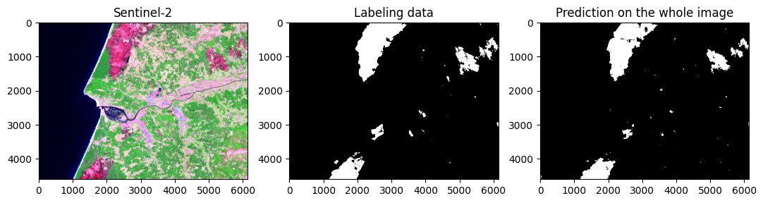
Reconstructing patches into a single patch is crucial to extract statistical metrics from the obtained predictions. This final step can be a challenge if you are working with large areas of land, which implies a large volume of patches to process. Furthermore, this step is an additional challenge if the patches are downloaded from GEE because there will be some columns and rows that will have to be filled in during the patch reconstruction process. This is because your study area will not exactly fit the dimensions of the patches to be downloaded.
Keep this in mind when you need to reconstruct the patches and then download them in some format such as ".TIF", for example.
| # reconstructing the whole image and labeling data
reconstructed_pred = unpatchify(predicted_patches, (num_patches_cols*patch_size, num_patches_rows*patch_size))
reconstructed_image = unpatchify(patches, (num_patches_cols*patch_size, num_patches_rows*patch_size, nbands))
reconstructed_labels = unpatchify(patches_labels, (num_patches_cols*patch_size, num_patches_rows*patch_size))
|
Visualizing the reconstructed image, predictions and labeling data in a single patch.
1
2
3
4
5
6
7
8
9
10
11
12
13
14
15
16
17
18
19
20
21
22 | # histogram with percentiles
def hist_percentile(arr_rgb):
p10 = np.nanpercentile(arr_rgb, 10) # percentile10
p90 = np.nanpercentile(arr_rgb, 90) # percentile90
clipped_arr = np.clip(arr_rgb, p10, p90)
arr_rgb_norm = (clipped_arr - p10)/(p90 - p10)
return arr_rgb_norm
orig_map = plt.colormaps['Greys']
reversed_map = orig_map.reversed()
img = reconstructed_image
fig, ax = plt.subplots(1, 3, figsize = (13,8))
rgb_patch = hist_percentile(np.dstack((img[:,:,9], img[:,:,6], img[:,:,2])))
ax[0].imshow(rgb_patch)
ax[0].set_title('Sentinel-2')
ax[1].imshow(reconstructed_labels, cmap = reversed_map)
ax[1].set_title('Labeling data')
ax[2].imshow(reconstructed_pred, cmap = reversed_map)
ax[2].set_title('Prediction on the whole image')
plt.show()
|