02-Preprocessing patches for burned area mapping

In this step patches downloaded from Google Earth Engine (GEE) will be preprocessed as input for applying the U-net architecture in order to map burned areas. We will kick off by reading TFRecod format from Google Drive, and finish with some patches visualizations using the scikit-eo Python package.

01. Libraries to be installed:

!pip install scikeo

02. Libraries to be used:

import json
import numpy as np
from scikeo.plot import plotRGB
import matplotlib.pyplot as plt
import matplotlib as mpl
from pathlib import Path
from google.colab import drive
import tensorflow as tf
from sklearn.preprocessing import StandardScaler

Count the number of cores in a computer:

import multiprocessing
multiprocessing.cpu_count()

Connecting to Google Drive: This step is very importante considering that the downloaded patches are inside Google Drive.

# Connect to Drive
drive.mount('/content/drive')

03. Reading patches dowloaded from Earth Engine

# prefix of patches
file_prefix = 'Port'

# Create a path to the exported folder
path = Path('/content/drive/MyDrive/Training_patches_512-512_Portugal/tile_17')

# creating a list of patches paths
paths = [f for f in path.iterdir() if file_prefix in f.stem]
paths, len(paths)

04. Display metadata for patches

Patch dimensions (pixels per rows, cols), patches per row and total patches are crucial for the unpatched process.

# load the mixer json
json_file = str(path/(file_prefix+'-mixer.json'))
json_text = !cat "{json_file}"

# print the info
mixer = json.loads(json_text.nlstr)
mixer

Number of patches per row and col is display in the following image:

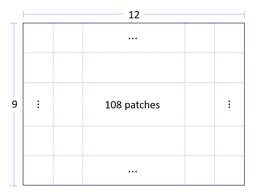
Getting patch dimensions an total patches:

# Get relevant info from the JSON mixer file
patch_width = mixer['patchDimensions'][0]
patch_height = mixer['patchDimensions'][1]
patches = mixer['totalPatches']
patch_dimensions_flat = [patch_width, patch_height]
patch_dimensions_flat, patches

05. Define the structure of your data

For parsing the exported TFRecord files, featuresDict is a mapping between feature names (recall that featureNames contains the band and label names) and float32 tf.io.FixedLenFeature objects. This mapping is necessary for telling TensorFlow how to read data in a TFRecord file into tensors. Specifically, all numeric data exported from Earth Engine is exported as float32.

Note: features in the TensorFlow context (i.e. tf.train.Feature) are not to be confused with Earth Engine features (i.e. ee.Feature), where the former is a protocol message type for serialized data input to the model and the latter is a geometry-based geographic data structure.

# bands names
bands = ['B2_median', 'B3_median', 'B4_median', 'B5_median', 'B6_median', 'B7_median', 'B8_median',
         'B8A_median', 'B11_median', 'B12_median', 'dNBR', 'label']

# list of fixed-length features, all of which are float32.
columns = [tf.io.FixedLenFeature(shape=patch_dimensions_flat, dtype=tf.float32) for b in bands]

# dictionary with names as keys, features as values.
features_dict = dict(zip(bands, columns))
features_dict

06. Parse the dataset

Now we need to make a parsing function for the data in the TFRecord files. The data comes in flattened 2D arrays per record and we want to use the first part of the array for input to the model and the last element of the array as the class label. The parsing function reads data from a serialized Example proto into a dictionary in which the keys are the feature names and the values are the tensors storing the value of the features for that example. (These TensorFlow docs explain more about reading Example protos from TFRecord files).

# parsing function
def parse_tfrecord(example_proto):
  """The parsing function.

  Read a serialized example into the structure defined by featuresDict.

  Args:
    example_proto: a serialized Example.

  Returns:
    A tuple of the predictors dictionary including the label.
  """
  return tf.io.parse_single_example(example_proto, features_dict)

Note that you can make one dataset from many files by specifying a list

patch_dataset = tf.data.TFRecordDataset(str(path/(file_prefix+'-00008.tfrecord.gz')), compression_type='GZIP')
ds = patch_dataset.map(parse_tfrecord, num_parallel_calls = 5)
ds

07. Patches as tensors

In this step, patches downloaded for GEE will be saved as a tensor with shape (a, b, c, d), 4D. Where a represents the number of patches, b and c represent the patch dimension and d represents the number of bands for each patch.

# number of bands
nbands = 11

# empty tensors
array_image = np.zeros((patch_width, patch_height, nbands)) # filas, columnas y n bandas
array_label = np.zeros((patch_width, patch_height, 1)) # filas, columnas y n bandas

# let's save patches in a list
Xl = [] # Sentinel-2 bands
yl = [] # Labeling data

# bands names
bands_image = ['B2_median', 'B3_median', 'B4_median', 'B5_median', 'B6_median',
               'B7_median', 'B8_median','B8A_median', 'B11_median', 'B12_median', 'dNBR']
bands_label = ['label']

# stacking images within a tensor
# len(paths)-1
for file in range(len(paths)-1):
  image_dataset = tf.data.TFRecordDataset(str(paths[file]), compression_type = 'GZIP')
  ds = image_dataset.map(parse_tfrecord, num_parallel_calls = 10)
  arr = list(ds.as_numpy_iterator())
  # for sentinel-2 bands
  for j in range(len(arr)):
    names = arr[j]
    for i, bnames in enumerate(bands_image):
      array_image[:,:,i] = names[bnames]
    Xl.append(array_image.copy())
  # for labeling data
  for j in range(len(arr)):
    names = arr[j]
    for i, bnames in enumerate(bands_label):
      array_label[:,:,i] = names[bnames]
    yl.append(array_label.copy())

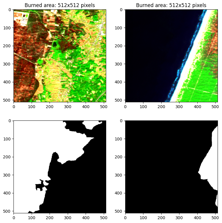
Then, patches can be converted to np.array. So, in total we have 108 patches with 512x512 pixels for both image and labeling data.

# list to array
X = np.array(Xl)
y = np.array(yl)

# print basic details
print('Input features shape:', X.shape)
print('\nInput labels shape:', y.shape)

Dealing with NaN values: In this step we are replacing NaN values for 0, in case our data contain Null values. This will allow computing matrix operations with deep learning architectures.

# replacing nan -> 0
X[np.isnan(X)] = 0

# replacing nan -> 0
y[np.isnan(y)] = 0

08. Normalizing data

Machine learning algorithms are often trained with the assumption that all features contribute equally to the final prediction. However, this assumption fails when the features differ in range and unit, hence affecting their importance.

Enter normalization - a vital step in data preprocessing that ensures uniformity of the numerical magnitudes of features. This uniformity avoids the domination of features that have larger values compared to the other features or variables.

Normalization fosters stability in the optimization process, promoting faster convergence during gradient-based training. It mitigates issues related to vanishing or exploding gradients, allowing models to reach optimal solutions more efficiently. Please see this article for more detail.

Z-score normalization:

Z-score normalization (standardization) assumes a Gaussian (bell curve) distribution of the data and transforms features to have a mean (μ) of 0 and a standard deviation (σ) of 1. The formula for standardization is:

Xstandardized = (X - μ)/ σ

This technique is particularly useful when dealing with algorithms that assume normally distributed data, such as many linear models.

Z-score normalization is available in scikit-learn via StandardScaler.

# normalizing data using scikit-learn
for i in range(X.shape[3]):
    band = X[:, :, :, i]
    band_normalized = StandardScaler().fit_transform(band.reshape(-1, 1)).reshape(108, 512, 512)
    X[:, :, :, i] = band_normalized

# Verifying dimensions (shape)
print("Normalized array:", X.shape)

Labeling data only has two values 0 and 1, which 0 means unburned and 1 burned area. According to your data, labeling data could have many values.

# details
print('Values in input features, min: %d & max: %d' % (np.min(y), np.max(y)))

09. Visualization of patch

Visualizing patches and labeling data using the scikit-eo Python package with the plotRGB function.

orig_map = plt.colormaps['Greys']
reversed_map = orig_map.reversed()

fig, ax = plt.subplots(2, 2, figsize = (9,9))

for i, idx in enumerate([17,15]):
  rgb = np.moveaxis(np.array(Xl)[idx,:,:,:], -1, 0)
  # satellite image (patches)
  plotRGB(rgb, bands = [10, 8, 3], title = 'Burned area: 512x512 pixels',
           stretch = 'per', ax = ax[0, i])
  # labeling data
  ax[1, i].imshow(y[idx,:,:,:], cmap = reversed_map)
  ax[1, i].get_xaxis().set_visible(True)
  ax[1, i].get_yaxis().set_visible(True)