03-Training and validation¶

01. Libraries to be installed:¶

!pip install patchify

02. Libraries to be used:¶

import random
import numpy as np
from scikeo.plot import plotRGB
import matplotlib as mpl
from sklearn.model_selection import train_test_split
from sklearn.metrics import accuracy_score, recall_score, precision_score, f1_score
from sklearn.metrics import confusion_matrix
import tensorflow as tf
from tensorflow import keras
from keras import models
from keras import layers
from keras.metrics import MeanIoU
from keras.utils import to_categorical
from keras import layers, Model
from patchify import patchify, unpatchify
from google.colab import drive

03. Training and testing¶

To train Machine Learning and Deep Learning models, 80% of the data could be used and 20% is used as validation of the trained model. But, sometimes this percetange could change, e.g., 50% for training and 50% for testing or 70% for training and the rest for testing, etc.

So, in this material, 80% will be used for traning. Getting training and testing data:

Xtrain, Xtest, ytrain, ytest = train_test_split(X, y, train_size = 0.6, random_state = None)

# visualizing the array dimensions
Xtrain.shape, Xtest.shape, ytrain.shape, ytest.shape

# unique classes
n_classes = len(np.unique(y))
# converts a class vector (integers) to binary class matrix
ytrain_catego = to_categorical(ytrain, num_classes = n_classes)
ytest_catego = to_categorical(ytest, num_classes = n_classes)

# visualizing the shape of the arrays
Xtrain.shape, Xtest.shape, ytrain_catego.shape, ytest_catego.shape

04. U-net architecture¶

To import or implement the U-Net model in Python, you usually need to define the architecture manually since U-Net is not part of the predefined architectures in libraries like TensorFlow or Keras. You can implement U-Net from scratch or use available third-party implementations.

Here is a basic example of how to define the U-Net architecture using Keras (with TensorFlow backend):

The following codes define a typical U-Net model with:

An encoding path (encoder) that reduces the dimensions using Conv2D and MaxPooling2D.
A decoding path (decoder) that restores the original dimensions using Conv2DTranspose.
Skip connections between the encoder and decoder layers to retain spatial information.

# U-net architecture
def unet_model(num_classes = 2, img_height = 256, img_width = 256, img_channels = 1):
    # Build the model
    inputs = layers.Input((img_height, img_width, img_channels))

    # Down-sampling path (Encoder): Contraction path
    conv1 = layers.Conv2D(64, 3, activation='relu', padding='same')(inputs)
    conv1 = layers.Conv2D(64, 3, activation='relu', padding='same')(conv1)
    pool1 = layers.MaxPooling2D(pool_size=(2, 2))(conv1)

    conv2 = layers.Conv2D(128, 3, activation='relu', padding='same')(pool1)
    conv2 = layers.Conv2D(128, 3, activation='relu', padding='same')(conv2)
    pool2 = layers.MaxPooling2D(pool_size=(2, 2))(conv2)

    conv3 = layers.Conv2D(256, 3, activation='relu', padding='same')(pool2)
    conv3 = layers.Conv2D(256, 3, activation='relu', padding='same')(conv3)
    pool3 = layers.MaxPooling2D(pool_size=(2, 2))(conv3)

    conv4 = layers.Conv2D(512, 3, activation='relu', padding='same')(pool3)
    conv4 = layers.Conv2D(512, 3, activation='relu', padding='same')(conv4)
    pool4 = layers.MaxPooling2D(pool_size=(2, 2))(conv4)

    # Bottleneck
    conv5 = layers.Conv2D(1024, 3, activation='relu', padding='same')(pool4)
    conv5 = layers.Conv2D(1024, 3, activation='relu', padding='same')(conv5)

    # Up-sampling path (Decoder): Expansive path
    up6 = layers.Conv2DTranspose(512, 2, strides=(2, 2), padding='same')(conv5)
    up6 = layers.concatenate([up6, conv4])
    conv6 = layers.Conv2D(512, 3, activation='relu', padding='same')(up6)
    conv6 = layers.Conv2D(512, 3, activation='relu', padding='same')(conv6)

    up7 = layers.Conv2DTranspose(256, 2, strides=(2, 2), padding='same')(conv6)
    up7 = layers.concatenate([up7, conv3])
    conv7 = layers.Conv2D(256, 3, activation='relu', padding='same')(up7)
    conv7 = layers.Conv2D(256, 3, activation='relu', padding='same')(conv7)

    up8 = layers.Conv2DTranspose(128, 2, strides=(2, 2), padding='same')(conv7)
    up8 = layers.concatenate([up8, conv2])
    conv8 = layers.Conv2D(128, 3, activation='relu', padding='same')(up8)
    conv8 = layers.Conv2D(128, 3, activation='relu', padding='same')(conv8)

    up9 = layers.Conv2DTranspose(64, 2, strides=(2, 2), padding='same')(conv8)
    up9 = layers.concatenate([up9, conv1])
    conv9 = layers.Conv2D(64, 3, activation='relu', padding='same')(up9)
    conv9 = layers.Conv2D(64, 3, activation='relu', padding='same')(conv9)

    # Output layer
    if num_classes == 1:
        outputs = layers.Conv2D(1, 1, activation='sigmoid')(conv9)  # Binary classification
    else:
        outputs = layers.Conv2D(num_classes, 1, activation='softmax')(conv9)  # Multi-class classification

    model = Model(inputs=[inputs], outputs=[outputs])

    return model

Keep in mind:

num_classes argument: This argument controls the number of output classes.
If num_classes=1, the model will use sigmoid activation for binary classification.
If num_classes>1, the model will use softmax activation for multi-class classification.
Output Layer:
For binary classification: Conv2D(1, 1, activation='sigmoid').
For multi-class classification: Conv2D(num_classes, 1, activation='softmax').

Now, you can use the num_classes argument to create either a binary classification U-Net or a multi-class classification U-Net.

# calling the model
model = unet_model(num_classes = 2, img_height = 512, img_width = 512, img_channels = 11)
#model.compile(optimizer='adam', loss=total_loss, metrics=metrics)
model.compile(optimizer='adam',
              loss='categorical_crossentropy',
              metrics=['accuracy'])
model.summary()

Verifying the input shape:

model.input_shape

05. Running the trained model¶

You'll now train the model for 220 epochs (i.e., 220 iterations over all samples in the Xtrain and ytrain_catego tensors), in mini-batches of 8 samples.

Hyperparameters used: - Number of epochs: epochs = 220 - Batch size: batch_size = 8

These hyperparameters can be modify according to your needs and computational capabilities.

# Run the model
history = model.fit(Xtrain,
                    ytrain_catego,
                    epochs = 220,
                    batch_size = 8,
                    verbose = 1)

Important!: How can we improve the accuracy?, There are some hyperparameters that you can modify in order to increase the accuracy of the model. - For example, epochs: Increasing the number of iterations is often a practice to improve the accuracy.

However, not always increasing this hyperparameter will lead to better accuracy or prediction of the models. It is important to find a balance to what extent it can affect on the final performance of our DL model. Do not go for overfitting or underfitting.

06. Monitoring during training¶

In order to monitor during training the accuracy of the model on data it has never seen before, you'll create a validation set by setting apart of n% samples from the original training data. You'll monitor loss and accuracy on the n% samples that you set apart. You do so by passing the validation data as the validation_data argument as follow:

# 10 percent for validation
history = model.fit(Xtrain,
                    ytrain_catego,
                    epochs = 220,
                    batch_size = 8,
                    validation_data = 0.1,
                    verbose = 1)

If you want to avoid this argument during training, you'll monitor loss and accuracy with the Xtrain and ytrain_catego tensors.

hist = history.history

epochs = range(220)

fig, axes = plt.subplots(figsize = (6,5))
ln1 = axes.plot(epochs, hist.get('accuracy'), marker ='o', markersize = 6,  label = 'Training acc')

axes2 = axes.twinx()
ln2 = axes2.plot(epochs, hist.get('loss'), marker = 'o', color = 'r', label = "Training loss")

# lengend
ln = ln1 + ln2
labs = [l.get_label() for l in ln]

axes.legend(ln, labs, loc = 'center right')
axes.set_xlabel("Num of epochs")
axes.set_ylabel("OA")
axes2.set_ylabel("Loss values")
axes2.grid(False)
plt.show()

Print the accuracy obtained on data it has never seen before with Xtest and ytest_catego:

test_loss, test_acc = model.evaluate(Xtest, ytest_catego)
print(f'test_loss: {test_loss}\ntest_acc: {test_acc}')

07. Saving and reading the model trained¶

The section below illustrates how to save and restore the model in the .keras format. - Please see this website https://www.tensorflow.org/tutorials/keras/save_and_load for more details.

# Save the entire model as a `.keras` zip archive.
model.save('/content/drive/MyDrive/00_PhD/models/Portugal/unet_model_6tiles.keras')

Reload a fresh Keras model from the .keras zip archive:

# Reading the model saved
model = tf.keras.models.load_model('/content/drive/MyDrive/00_PhD/models/Portugal/unet_model_6tiles.keras')

# Show the model architecture
model.summary()

Now you can verify the expected dimensions for input

# expected dimensions for input
model.input_shape

08. Accuracy assessment of burned area mapping¶

To evaluate the accuracy of classifications map, indicators such as overall accuracy (this was obtained from the error matrix), Recall, Precision, F1-score and Intersection-Over-Union were used.

# define classes
class_names = ['burned', 'unburned']

# compute predictions
y_pred = model.predict(Xtest)
y_pred_argmax = np.argmax(y_pred, axis = 3)
y_test_argmax = np.argmax(ytest_catego, axis = 3)

Overall Accuracy

# Overall accuracy obtained
print("overall accuracy: {:.4f}".format(accuracy_score(y_test_argmax.flatten(), y_pred_argmax.flatten())))

Recall

# Recall obtained
print("Recall obtained: {:.4f}".format(recall_score(y_test_argmax.flatten(), y_pred_argmax.flatten())))

Precision

# Precision obtained
print("Precision obtained: {:.4f}".format(precision_score(y_test_argmax.flatten(), y_pred_argmax.flatten())))

F1-score

# F1-score obtained
print("F1-score obtained: {:.4f}".format(f1_score(y_test_argmax.flatten(), y_pred_argmax.flatten())))

IoU (Intersection-Over-Union)

It is a common evaluation metric for semantic image segmentation. How does it work?

confusion matrix = [(1, 1), (1, 1)]

sum_row = (2, 2), sum_col = (2, 2), true_positives = (1, 1)

iou = true_positives/(sum_row + sum_col - true_positives)

iou = [0.33, 0.33]

https://www.tensorflow.org/api_docs/python/tf/keras/metrics/IoU

# Using built in keras function for IoU
n_classes = len(np.unique(y))
IOU_keras = MeanIoU(num_classes=n_classes)
IOU_keras.update_state(y_test_argmax, y_pred_argmax)
print("Mean IoU =", IOU_keras.result().numpy())

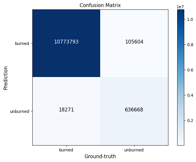
09. Confusion matrix¶

Let's plot Confusion Matriz

def plotConfusionMatrix(y_test , y_pred , text_size = 12, classes = None , ax = None):

  if ax is None:
        ax = plt.gca() # get current axes

  # Create the confusion matrix from sklearn
  cm = confusion_matrix(y_test , y_pred)
  threshold = (cm.max() + cm.min()) /2

  # Number of clases
  n_classes = cm.shape[0]

  # Drawing the matrix plot
  b = ax.matshow(cm , cmap = plt.cm.Blues)
  bar = plt.colorbar(b)

  # Set labels to be classes
  if classes:
    labels = classes
  else:
    labels = np.arange(cm.shape[0])

  # Label axes
  ax.set(title ='Confusion Matrix', xlabel = 'Ground-truth' ,
         ylabel = 'Prediction', xticks = np.arange(n_classes),
         yticks = range(n_classes), xticklabels = labels , yticklabels = labels)
  # Set the xaxis labels to bottom
  ax.xaxis.set_label_position('bottom')
  ax.xaxis.tick_bottom()

  # Adjust the label size
  ax.yaxis.label.set_size(text_size)
  ax.xaxis.label.set_size(text_size)
  ax.title.set_size(text_size)
  ax.grid(False)

  # Plot the text on each cell
  for i in range(cm.shape[0]):
    for j in range(cm.shape[1]):
      ax.text(i,j, f'{cm[i,j]}',
               horizontalalignment = 'center' ,
               color = 'white' if cm[i , j] > threshold else 'black',
               size = text_size)

fig, ax = plt.subplots(figsize = (8,6))
plotConfusionMatrix(y_test_argmax.flatten(), y_pred_argmax.flatten(), classes = class_names)

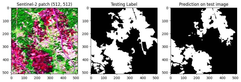
10. Predicting for one patch¶

test_img_number = random.randint(17, len(Xtest))
test_img = Xtest[test_img_number]
ground_truth = y_test_argmax[test_img_number]
test_img_input=np.expand_dims(test_img, 0)
prediction = (model.predict(test_img_input))
predicted_img=np.argmax(prediction, axis=3)[0,:,:]

# histogram with percentiles
def hist_percentile(arr_rgb):
  p10 = np.nanpercentile(arr_rgb, 10) # percentile10
  p90 = np.nanpercentile(arr_rgb, 90) # percentile90
  clipped_arr = np.clip(arr_rgb, p10, p90)
  arr_rgb_norm = (clipped_arr - p10)/(p90 - p10)
  return arr_rgb_norm

orig_map = plt.colormaps['Greys']
reversed_map = orig_map.reversed()

fig, ax = plt.subplots(1, 3, figsize = (12,8))

rgb_patch = hist_percentile(np.dstack((test_img[:,:,9], test_img[:,:,6], test_img[:,:,2])))
ax[0].imshow(rgb_patch)
ax[0].set_title('Sentinel-2 patch (512, 512)')
ax[1].imshow(ground_truth, cmap = reversed_map)
ax[1].set_title('Testing Label')
ax[2].imshow(predicted_img, cmap = reversed_map)
ax[2].set_title('Prediction on test image')
plt.show()