Get Started¶

This guide presents a specialized workflow for mapping burned areas using the Normalized Radar Burn Ratio (NRBR) and Deep Learning (DL), with a focus on Mediterranean forests and Portugal's devastating 2017 wildfire season. The methodology leverages Sentinel-1 SAR data and a U-Net model to overcome limitations of optical-based indices in cloud-prone environments.The process is based on Google Earth Engine (GEE) for data processing and TensorFlow for model training.

Content¶

01. NRBR in Action: Portugal Case Study

02. Workflow based on using GEE and Google Colab

03. Data Preparation using GEE

04. Deep Learning Model (U-Net Architecture)

05. Burned area prediction

01. NRBR in Action: Portugal Case Study¶

In 2017, central Portugal experienced one of its most devastating wildfire seasons, with over 217,000 hectares burned. Two 50×50 km tiles, hereafter referred to as Tile1 and Tile2, were selected for analysis.

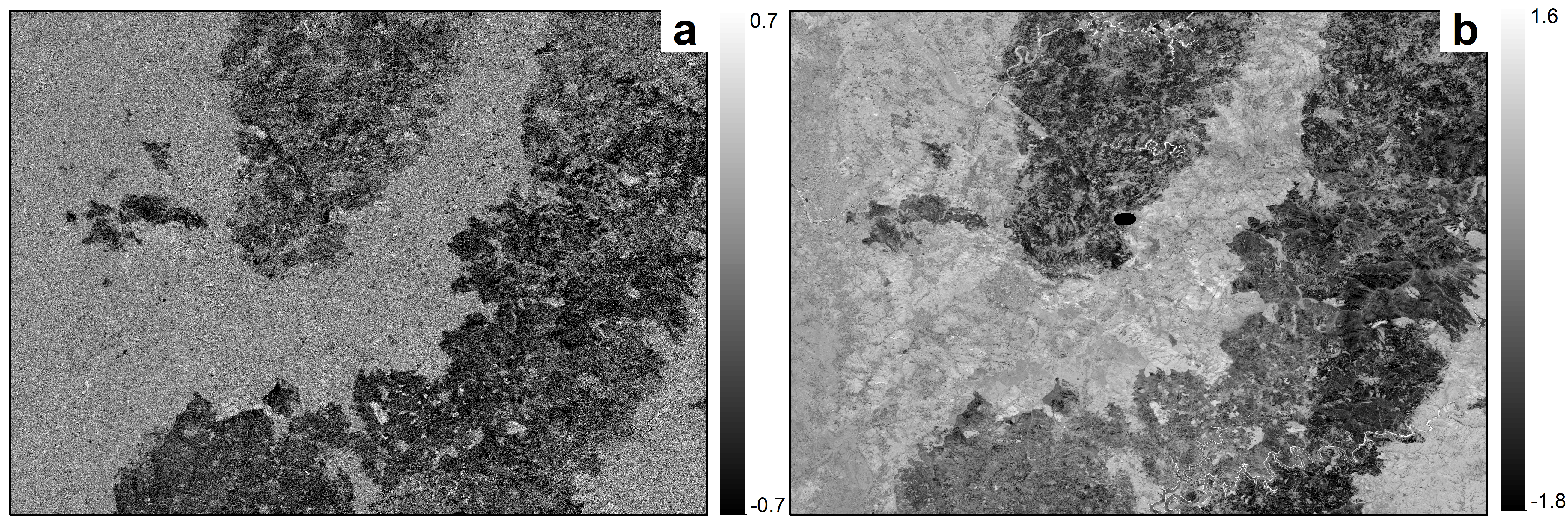
Optical indices like dNBR (delta Normalized Burn Ratio) (panel b) are widely used for burned area mapping but fail under clouds or smoke. NRBR (panel a), a radar-based index, overcomes this limitation by using Sentinel-1’s SAR data, which penetrates atmospheric obstructions.

Key Insight:

Sensitive to vegetation changes: Burned areas show negative NRBR values (unburned: positive values).
Combining ascending (ASC) and descending (DSC) orbits improves detection accuracy.
All-weather capability: radar Works through clouds, smoke, and darkness (unlike optical indices).

02. Workflow based on using GEE and Google Colab¶

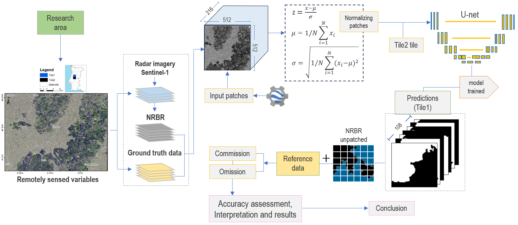
To map burned areas using the NRBR derived from Sentinel-1 radar imagery, one potential approach involves downloading input patches (e.g., affected and reference areas) from GEE. The workflow suggests leveraging a DL model architecture, where the model is trained on one set of patches (e.g., Tile2) and subsequently applied to predict burned areas in another (e.g., Tile1). The trained model, implemented in frameworks like TensorFlow on Google Colab, can generate predictions, followed by accuracy assessment and interpretation of results. This methodology highlights the flexibility of using cloud-based tools (GEE, Colab) for efficient burned-area mapping.

03. Data Preparation using GEE¶

Downloading patches from GEE and Python¶

Patches for DL architectures are crucial for land cover disturbance mapping, including burned area mapping. A good option is to download from GEE using the Python API or JavaScript, whichever you are comfortable with.

A specific tile with 50x50km (i.e., 25 million pixels) from Portugal during the 2017 year will be downloaded. Labeling data known as ground truth for the same tile will be downloaded as well.

Sentinel-1 Input:
- Pre-fire: Average of 13 scenes (15 May – 15 June 2017) to reduce speckle noise (GEE’s mean() reducer).
- Post-fire: Average of 12 scenes (15 October – 15 December 2017).
- Orbits: Combine ascending (ASC) and descending (DSC) modes for higher accuracy.
Download: Export as TFRecords (patches of 512×512 pixels at 10m resolution).

Patch Preprocessing (Google Colab)¶

Before model training, the input patches were standardized using scikit-learn's StandardScaler, which applies Z-score normalization by centering the data (subtracting the mean) and scaling it by the standard deviation. This preprocessing step improves training stability and ensures better generalization across different geographic tiles. The entire workflow—from patch normalization to model training—was executed in Google Colab using TensorFlow, leveraging its computational efficiency for seamless integration of remote sensing data into deep learning pipelines.

Normalization: Normalized NRBR values.
Split Data:
- Training: 108 patches from Tile2.
- Testing: 108 patches from Tile1 (independent tile).
- Labels: Rasterized ground truth (10m resolution) from Portuguese government (DGT).

04. Deep Learning Model (U-Net Architecture)¶

Key Parameters:

Depth: 4-5 encoder/decoder layers (with skip connections).
Input: NRBR patches (512×512×1).
Training:
- Epochs: 200 (combined ASC+DSC).
- Batch Size: 8.
- Optimizer: Adam.
- Loss: Categorical cross-entropy.
- Output: Binary mask (softmax activation).

05. Burned area prediction¶

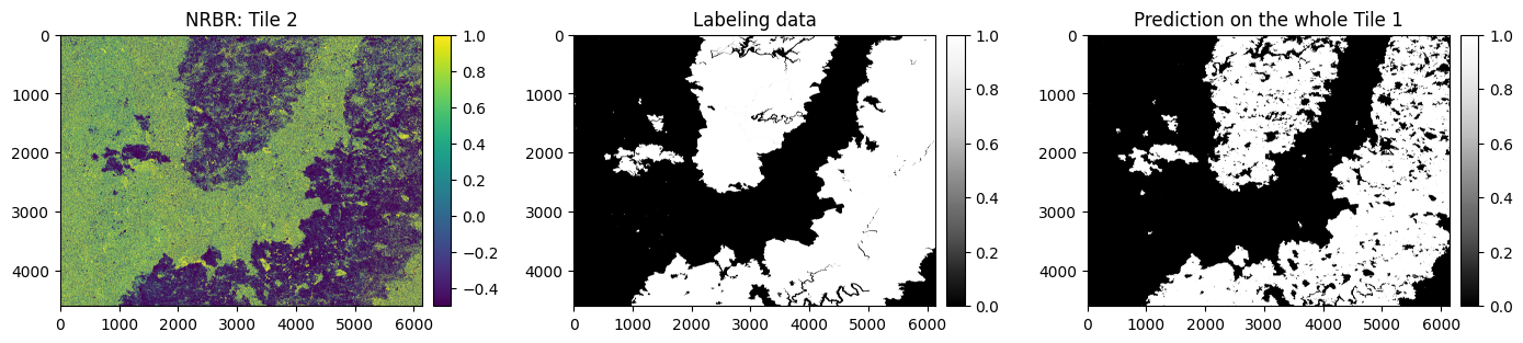
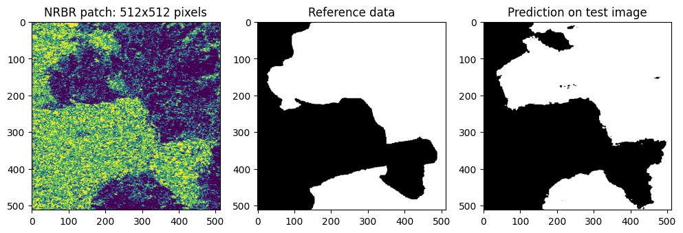
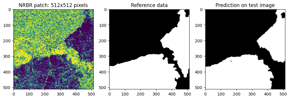
These 512×512-pixel NRBR patches demonstrate the effectiveness of our radar-based burned area detection system. Each patch compares: (1) the NRBR input (showing negative values for burned areas), (2) the ground truth reference data from Portuguese authoritiesthe, and (3) the U-Net model's prediction. The model, trained on ascending and descending Sentinel-1 orbits, achieves higher overall accuracy by leveraging NRBR's sensitivity to vegetation structure changes. Notably, it maintains high precision while reducing omission errors - critical for reliable fire monitoring. The consistent alignment between predictions and reference data across these samples highlights NRBR's advantage over optical methods, mainly in cloud-affected regions.

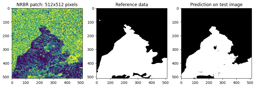
Predicting for one patch¶

Predicting on the whole Tile 1¶

The integration of ascending and descending Sentinel-1 orbits NRBR demonstrated superior performance for burned area mapping compared to single-orbit.

Table 1. Accuracy metrics comparison for NRBR using single-orbit (ASC/DSC) vs. combined Sentinel-1 acquisitions¶

Metric	ASC Only	DSC Only	Combined (ASC+DSC)	Improvement
Overall Accuracy (OA)	0.896	0.894	0.921	+2.7%
Recall	0.812	0.801	0.858	+5.7%
Precision	0.970	0.978	0.977	±0.0%
IoU	0.810	0.806	0.852	+4.6%
Omission Errors (%)	18.30	19.90	14.20	-6.0%
Commission Errors (%)	3.40	2.20	2.30	-1.1%
Dice Coefficient	88.27	88.12	91.32	+3.2%

Key Findings:
1. Combined orbits reduce omission errors by 6.0% compared to ASC/DSC-only.
2. Best balance: Highest recall (0.858) while maintaining precision >97%.
3. Optimal segmentation: Dice=91.32 and IoU=0.852 outperform single-orbit approaches.